There are several instances when having a scroll bar linked to an Excel chart can come in handy – it’s a great way to make your chart dynamic and can really enhance the functionality of an Excel dashboard. On this page, we’ll describe how to add a scroll bar to your Excel chart – in Excel 2007. We’ll provide an example file, created using the steps, with the completed chart and scroll bar.  This will allow you to check your result against ours or use the example in your own project.

How to Add a Scroll Bar in Excel

Scroll Bar Example Download

Download 53.50 KB 745 downloads

Step 1

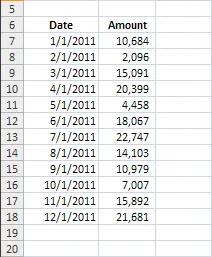
Determine where your data set is going to be because we’re going to be using dynamic formulas. In our example, we have a column for Date, and one for Amount. Our data set is set up as shown below. The thing to consider at this point is how many rows will ultimately end up being a part of what needs to be graphed (this will impact future steps).
Excel Scroll Bar
Step 2

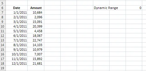
Next, determine where you want your dynamic range – this is the cell that is ultimately going to drive the data that’s reflected within your chart. Typically, I like to put this cell somewhere that will not show up when the data & chart are printed, and will not be deleted. If you simply want it hidden, you can always cut and paste it under your chart once the chart has been created. For this example we set ours up like this:
Excel Scroll Bar

Step 3

Excel Scroll Bar
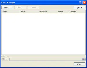
Now we’re going to create a ‘Named Range’ for our chart. To do this, push Ctrl+F3 (which brings up ‘Name Manager’) and select ‘New’.
Excel Scroll Bar
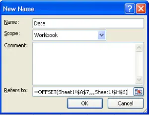
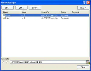
The ‘New Name’ dialog box will come up – enter ‘Date’ as the name and this formula =OFFSET(Sheet1!$A$7,,,Sheet1!$H$6) and select OK (second picture). The ‘Name Manager’ will come up again and select ‘New’ again.
Excel Scroll Bar
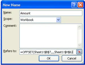
Enter the information shown here. Select ‘OK’ and close the Name Manager. You can read more about the offset formula here. We’re not going to get into the details of this function here.
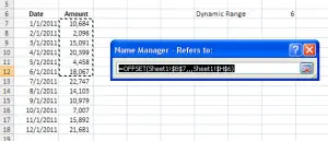
Tip – You can check to see if the formula you’ve entered in the name manager is working properly by clicking as shown in the picture to the right
Excel Scroll Bar
We entered the value of 6 in the dynamic range cell, so 6 values in the Amount column should be shown as reflected here.
Excel Scroll Bar

Step 4

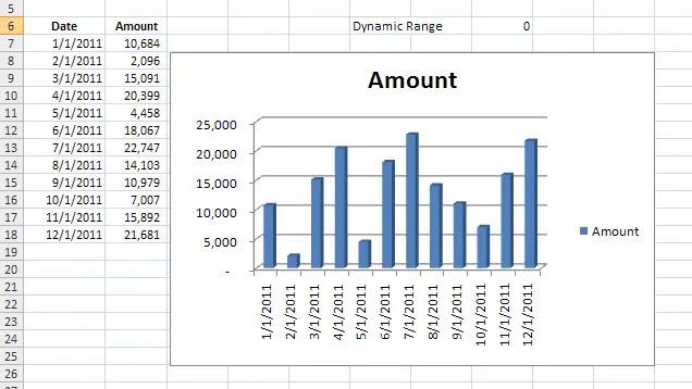
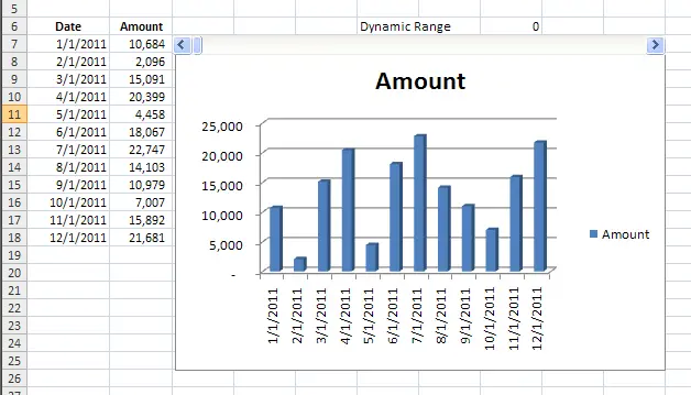
Here we’ll insert the chart. For this example, we’ve selected a 3-D bar chart. To add the chart, select cell A7 > select the ‘Insert’ ribbon > ‘Column’ > ‘3-D Column’. The following chart will be created.
Excel Scroll Bar

Step 5

The last piece we need to include is the scroll bar. To do this, first enable your ‘Developer’ ribbon (Excel Orb > Excel Options > Popular > Check the box for ‘Show Developer tab). Under the ‘Developer’ ribbon choose Insert > Scroll Bar. Then, insert the scroll bar where you want it – we put it right over the chart.
Excel Scroll Bar

Step 6

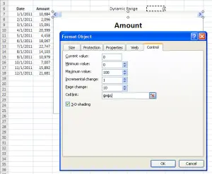
Now it’s time to tie all of the pieces together. First, right click on the scroll bar, choose ‘Format Control’. On the ‘Control’ tab, enter $H$6 in the ‘Cell Link’ box. Before moving forward, ensure that a value larger than zero is entered into the Dynamic Range cell.
Excel Scroll Bar
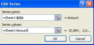
Now, left click on the chart, and under the ‘Chart Tools’ ribbon select ‘Design’ then ‘Select Data’. Select ‘Amount’ and ‘Edit’; the ‘Edit Series’ is displayed (complete as shown in the picture).
Excel Scroll Bar
Lastly, choose ‘Edit’ under the ‘Horizontal Axis Labels’ (complete as shown in the 3rd picture).
Excel Scroll Bar

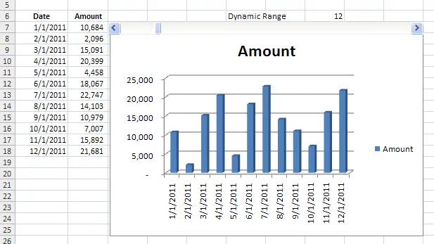
You’re Done!
Excel Scroll Bar