What is the Offset Function?
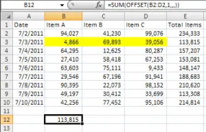
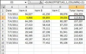
The offset function is a powerful Excel formula, the purpose of which is to return a single value or a range of values that is a given number of rows or columns from a specified reference (i.e. a specific cell – your starting point). This function is particularly useful when we don’t know the exact location or range needed (i.e., when the output needs to be dynamic or is dependent on other variables). This will start to make more sense as we go through examples.
The offset function is great for dynamic sums, implementing a scroll bar into a chart, dynamic charts, dashboards, named ranges, use with other functions such as the Match function, and the list goes on.
Excel’s Offset Function
The Basics
The formula is =Offset(Reference,Rows,Cols,Height,Width)
- Reference – this is where you want to base the offset, the starting location. It can be a single cell or a range of cells. There must be a value here, this is the only part of the offset function that requires a value.
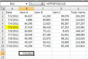
- Rows – is the number of rows (up or down) you want the upper-left cell of the result to refer to. A positive number moves down, negative moves up. If rows do not need to change, you can leave this blank or use a “0”.
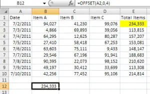
- Cols – is the number of columns (left or right) you want the upper-left cell of the result to refer to. A positive number moves right, negative moves left. If columns do not need to change, you can leave this blank or use a “0”.
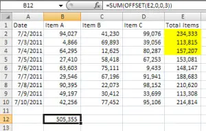
- Height – the number of rows you want to be in the result, by leaving this unused, the result will be the same height as the original reference. If you’re not using either height or width, the rest of the formula can be left blank, or you can use “0”.
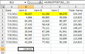
- Width – the number of columns you want to be in the result, by leaving this unused, the result will be the same width as the original reference. If you’re not using either height or width, the rest of the formula can be left blank, or you can use “0”.
Examples of the Offset Function
Each example is included within a tab of the download below – download the file to see how the function works and make modifications…the best way to learn. The first 5 examples are intended only to demonstrate what the offset function does, not best practices. As a best practice, formulas should be made as dynamic as possible – they shouldn’t need to be updated frequently. See the example in Tab 6 for a dynamic use of this formula.
Offset Function Example Download
Download 116.50 KB 757 downloadsOffset using Rows only – Tab 1
Offset using Height only – Tab 3
Offset using Width only – Tab 4
Offset using a Range for the Reference – Tab 5
Offset Function made Dynamic – Tab 6
Other Uses of the Offset Function Found on this Site
We’ve used the offset function in some of the templates uploaded on this website. If you would like to download the excel templates and see some more real world uses of this fantastic function, please click on the links below, or see the offset function used for Dynamic Printing.
