Automatically Alternate Row Coloring in Excel
Two Ways to Alternate Row Coloring in Excel
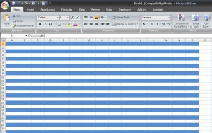
If you’re using excel 2007 or 2010, probably the quickest and easiest way to get automatically alternate row coloring is by using Excel’s built-in table feature. However, there are several instances when the solution calls for something other than an Excel table. In this article, we’re going to cover a very simple, yet effective way to automatically alternate row coloring within an Excel spreadsheet. We’ll use 3 concepts:
- Conditional Formatting
- The MOD function
- The ROW function
Automatically Alternate Row Coloring Download
Download 38.00 KB 480 downloads
The Short Answer
For those of you who don’t need a detailed step-by-step how-to, here you go:
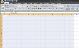
- Highlight the area of interest
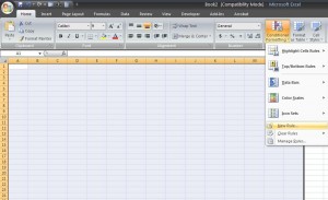
- Go to the conditional formatting section in the ribbon and select new rule
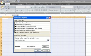
- Use the formula =MOD(ROW(),2)=1 and then set your preferences
Step-by-Step Instructions with Screen Shots
How does this formula work? The first thing that happens is that the =ROW() formula identifies the row number (i.e., 1 = 1, 2 = 2, etc). Then the MOD function divides the row number by a divisor, in this case 2 and returns either a “0” for even rows or a “1” for odd rows. Because we set the formula = 1, when that’s true, the conditional formatting is active. Change this formula to be less than 1, =MOD(ROW(),2)=0, if you wanted all even rows highlighted.
